How does storage organisation affect query performance?

Despite great efforts to separate interface from the implementation (like SQL), the pesky details always come up important when deploying to production, either when performance does not meet expectations or during error handling. The Amazon Redshift service Is not different and knowing data organisation – both on cluster and local level – is crucial when designing a performant database.

Abstract

Redshift stores data in two-level partitioning structure:

1. All data is divided into slices (partitions), each slice is stored on one node. Slices are controlled by distribution style.

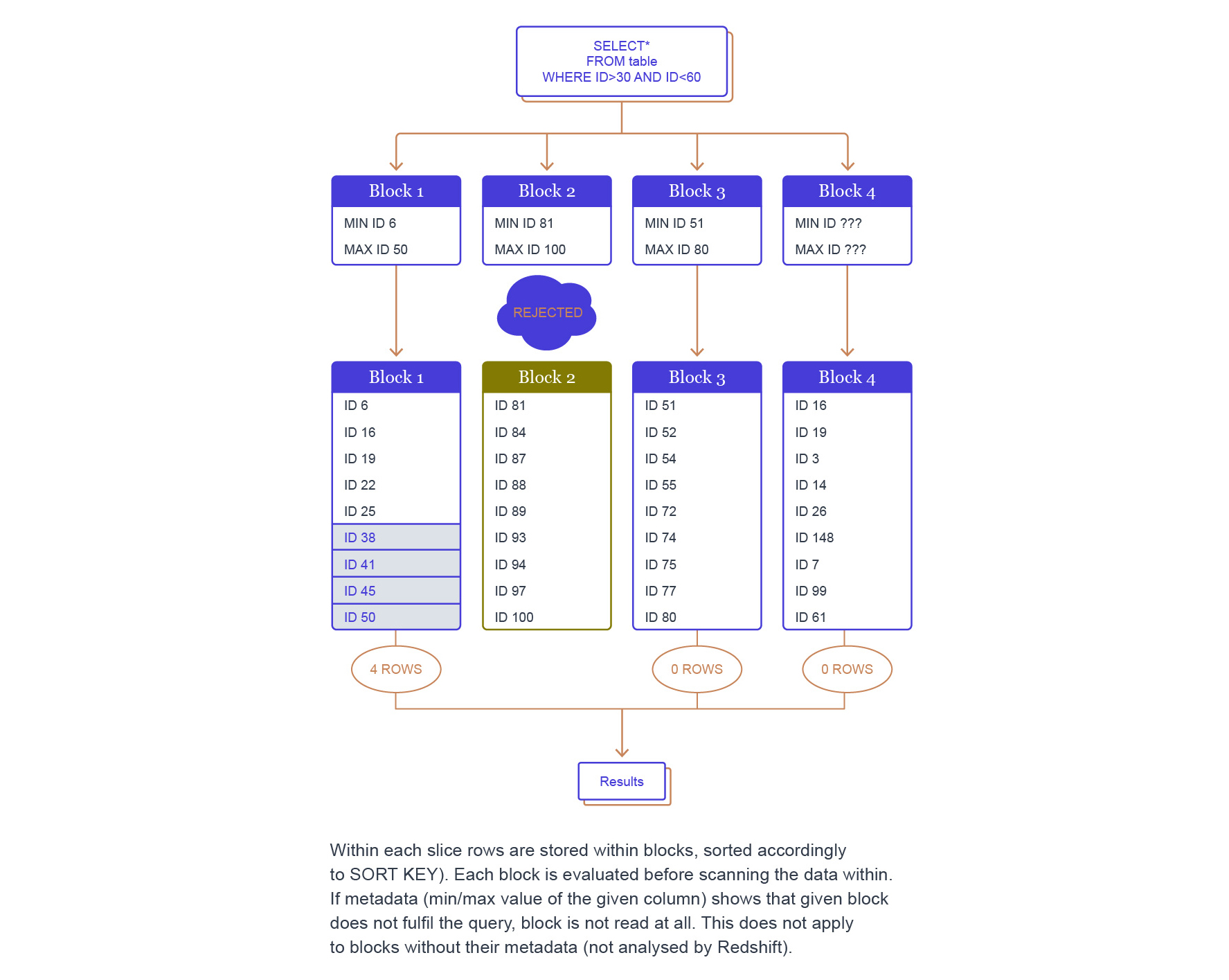
2. Slices are stored in data blocks, 1 megabyte per block. Each block comes with metadata (min & max value of a column in the block) that can be used by the master node to skip (or not) the block when executing a query.

You may want to take advantage of manual partitioning to achieve better cluster performance:

1. Distribution should be aligned to expected joins and groupings, to keep both operations local to a worker node (for each partition). Therefore distribution style should go along with JOIN predicates and GROUP BY columns.

2. Sorting key also determines the contents of the data blocks on nodes. Using the correct key may increase the number of data segments not read, increasing efficiency of users’ queries. Looking into data distribution in Redshift blocks for WHERE predicate columns may be helpful.

Efficient big data processing

How to process data quickly? There are a few guidelines that are useful even outside RS scope.

1. Process only the relevant data – do not read what you do not need.

2. Keep processing as close to the data as possible.

3. Keep the node load even and manageable.

Now let’s see how we can achieve the above points by correctly setting the keys.

Distribution style

Most big data tools work on partitioned data – Redshift is not different. User can specify one of  three options:

1. EVEN style, which randomly picks a slice for each node. This choice heavily optimizes balance among the slices (and thus nodes), but leaves no room to optimize joins and aggregations.

2. ALL style meant for small data sets (master data, dictionaries, etc.). This option puts the whole table on each node. All joins against all-distributed tables are local to each node.

3. KEY style, where the DBA picks the column for data distribution: same key means same slice. This allows making joins and group-bys local for each splice, but DBA must make sure that data is partitioned evenly and splices would not blow up nodes.

The correct distribution is one that goes best against SELECT queries while preserving good balance across slices. In most cases it means using KEY distribution, for example:

Joins – using KEY in both tables to colocate by join keys.
This will keep joined data on the same splice and eliminate the need to send rows across nodes.

Query involving GROUP BY clause – KEY by group key column(s).
It allows each aggregate to be calculated on only one splice each.

Query with WHERE predicate – KEY by predicate column(s).
If the query does not contain joins nor grouping and predicate columns group columns into nice, even partitions – they can be used to speed up a SELECT query.

Sorting: querying, loading and vacuuming

Locally on a splice Redshift organizes data into blocks – each one is a part of data of a specific column and  is described by min & max value in the zone map (if applicable). This means some of the blocks can be discarded without even opening their data files – every min-max range is outside WHERE predicate.

Accessing zone information

Redshift stores zones metadata is somewhat buried in the system tables and views. 

Use STV_BLOCKLIST and STV_TBL_PERM tables

SELECT * FROM STV_BLOCKLIST, STV_TBL_PERM

WHERE STV_BLOCKLIST.tbl = STV_TBL_PERM.id

     AND STV_BLOCKLIST.slice = STV_TBL_PERM.slice

     AND STV_TBL_PERM.name = '<table name here>'

     AND STV_BLOCKLIST.col = <column ord here>;

Columns (with their order) can be checked in SVV_REDSHIFT_COLUMNS (it cannot be joined with the previous query, though – mixing tables from master node with ones from compute nodes results in not-so-informative ERROR: 0A000: Specified types or functions (one per INFO message) not supported on Redshift tables).

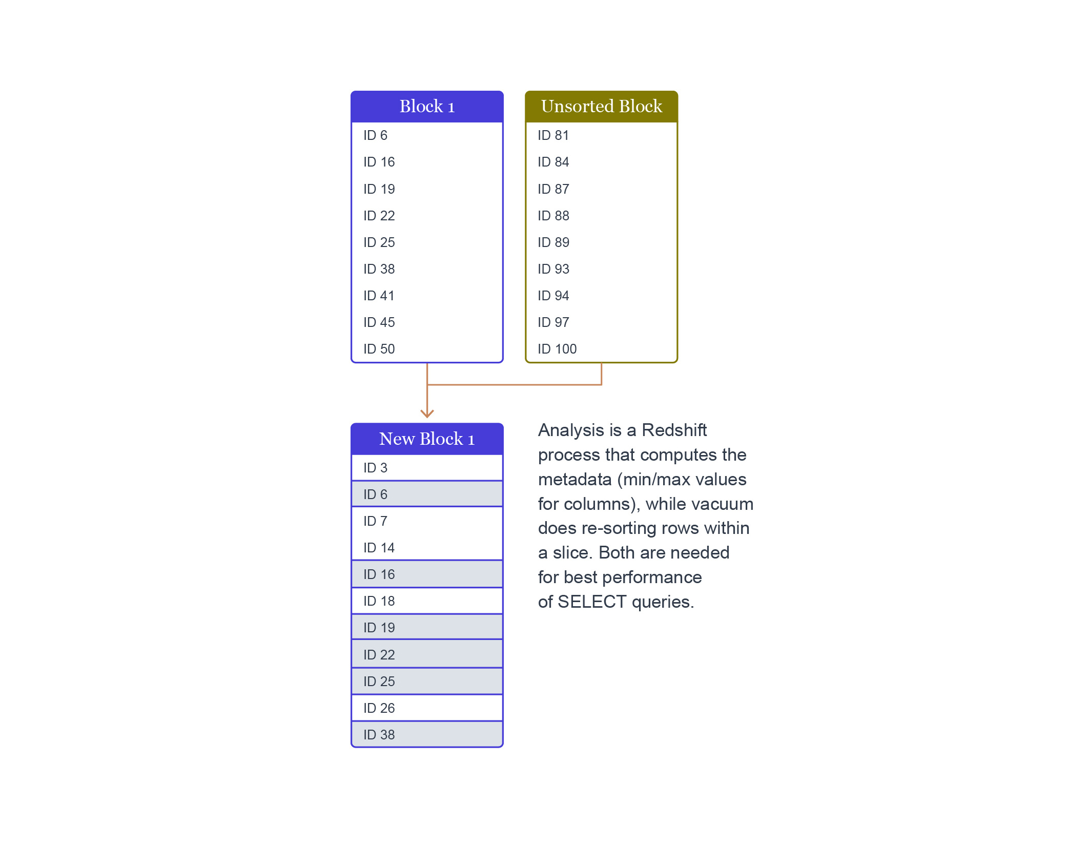
SELECT * FROM SVV_REDSHIFT_COLUMNS WHERE table_name = ‘<table name>’;

The block min-max information is calculated during execution of ANALYZE, though the command may be issued implicitly by RS itself (as noted in the documentation).

Note on analysis & vacuum

For frequently updated / modified tables one should use custom sort keys with caution. During data loading all data is appended to new, unsorted blocks (where block map is not computed yet). Using a very selective sorting key may hinder data loading – blocks will need to be recomputed to accommodate new rows. Good examples for sorting keys are:

• stable and low cardinality enumerations,
• auto-incremented IDs,
• creation or insert timestamps.

What should not be used as a part of sorting key:

• often mutated fields,
• most IDs and UUIDs.

Conclusion

1. Table schema and keys have to be aligned with queries that will be used on them, as RS is even more dependent on data layout than standard RDBMS deployments.

2. Distribution style EVEN is very rarely better than KEY one, especially in case of tables used in joins.

3. Sorting may speed up queries with selective predicates – as long as it does not hinder data loading.